

No matter what industry you work in, spreadsheets are pretty awesome. But sharing spreadsheets with multiple people is hard. How do you make it easy for other people to explore your data without getting lost in the filters?
One way to make filters more visible is to build a dashboard page that dynamically updates from the basic data set using a view in a specialized tab.
Let’s build a viewer for a spreadsheet in Google Sheets. We’ll take some standard data, build date filters and a couple of other dynamic filters, and use the QUERY function in Google spreadsheet.
How does this work?
This spreadsheet dynamically builds filters to change the view of the data. Most of this will happen automatically, and there are a few items you’ll need to customize.
What data should we use?
In this example, we use sample opportunity data from Salesforce, and copy it into an “ExampleData” tab. We use a helper tab called “ListData” to find sample columns (this supports up to 26 columns) and creates a list of values for our filters.
On the ListData tab, in A1 we find the column names by using this function:
=query(ExampleData!1:1,”Select * limit 1″)
This results in the columns we need, arranged as columns in our ListData tab, e.g. “Opportunity Owner” in Column B.
Row 2 of the ListData tab tells us the values for each column. Because the column in the ListData tab is in the same place as the column in the ExampleData tab, the same function works for all the columns in the row.
=ifError(unique(query({ExampleData!2:1000},”select Col” & Column() & ” where Col” & Column() & “!=””,0)),””)
The function writes out the unique values so we can use them in the Viewer as a Validation criteria for a filter.
How do we turn this into a viewer?
To turn this data into a viewer, we need to:
- Write as many columns as there are columns in the data set.
- Create a “filter”, which is essentially a cell containing a list with a validation rule showing us the expected values in that field in the dataset.
- Depending on the “filters” that are chosen by the viewer, write a dynamic SQL clause to show the relevant rows of the data set when a filter or filters are chosen.
To count the columns in the data set, we need a helper function that will tell us the column number matching the index of the rightmost column containing data.
Note: this technique works only with string data. If you want to filter on date values or numbers, we would need to update the spreadsheet to alter the query (email me if you’re interested: blog@gregmeyer.com)
This formula uses ARRAYFORMULA and LOOKUP to find the rightmost column in row 1 of the ListData set (you could use either the headers from the original ExampleData or the ListData as they are identical). In our example, we have 9 columns.
=match(ArrayFormula(LOOKUP(2,1/(ListData!A1:1>0),ListData!A1:1)),ListData!1:1,0)
For each of the nine columns, we need to create two rows:
- The first row, which is the columns in the ListData array.
- The second row, which is an empty cell with Data Validation.
For the first row, we use a trick to reference an array of 9 columns. The INDIRECT function creates a range between A1 (the first column of headers on the listData tab) and A9 (the last column in the set). The CHAR function lets us count up from A to I using the good old ASCII table.
Here’s the formula that does the work:
=indirect(“listData!”&”A1:” & Char(65+B1) & “1”)
The second row simply uses this Data Validation to select the corresponding set of values from the ListData tab. Viewer!A3 uses ListData!A2:A, Viewer!B3 uses ListData!B2:B, etc. You will need to make sure this data validation is in place for each column.
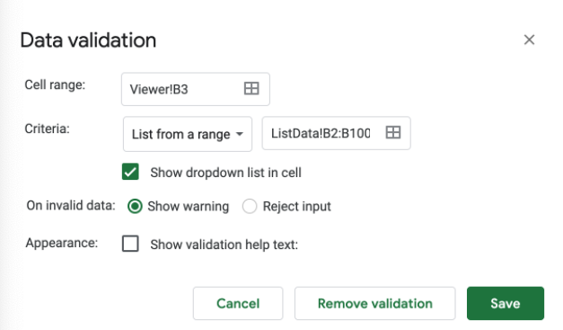
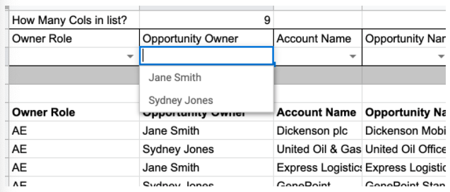
Here’s what that looks like when the validation is in place, creating a “drop-down” view of the data values from that column:
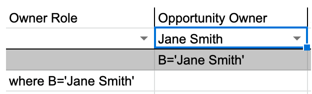
In A4, we do a bit more magic to JOIN together the various filter conditions so that we can feed them to the QUERY function.
=if(len(A3),Char(64+Column(A3)) &”='”&A3&”‘”,””)
This means that if we select “Jane Smith”, the following things happen. Column B is set to equal ”‘Jane Smith” and the compound query statement includes “Where B=’Jane Smith’”.
There’s one more piece of formula magic here. If you don’t specify a filter for each column, how do you only include the columns that are filtered in your QUERY?
Enter the JOIN and FILTER functions. Note that A4:I4 is the range of the columns we want to search. You’ll need to adjust I4 if you have more or fewer columns in your sample set.
=ifError(“where ” & join(” AND “,FILTER((A4:I4), NOT(A4:I4=””))),””)
When we select Opportunity Owner of “Jane Smith” and Stage of “Prospecting”, we end up with a result of:
where B=’Jane Smith’ AND E=’Prospecting’
As the empty fields are ignored.
How do we pull this all together?
Cell A6 finishes the viewer by selecting everything in the ExampleData data set except if there is a WHERE condition specified in A5 (because we selected some filters).
=query(ExampleData!1:1000,”select * ” & if(len(A5),” ” &A5,””))
This means that when no filters are selected, it runs an empty query. If filters are selected, the query is run with the WHERE clause we specified.
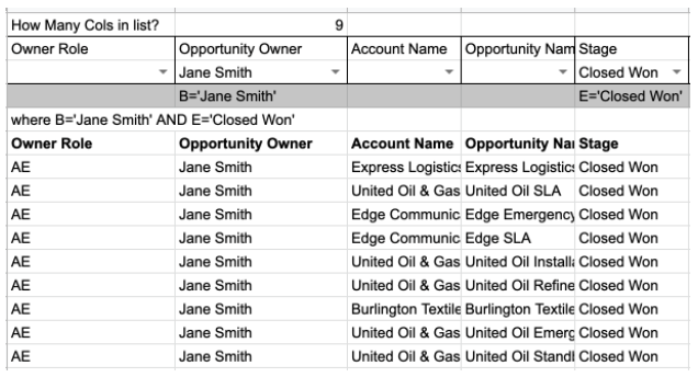
When we want to find the Closed Won opportunities for Jane Smith, we see only the nine rows that are relevant.
If we run the viewer with no filters, we see all 31 rows.
Here’s a link for you to make a copy of the spreadsheet. Happy viewing!
AUTHOR BIO

Greg makes data quality better for the go-to-market team at Redis Labs. From Leads to Contacts to Accounts, he’s responsible for resolving duplicates, building systems to improve quality and enrich data, and providing excellent service to the team. Greg lives in the beautiful Pacific Northwest near Seattle, Washington.